Welcome back! In the first post of this series, we learned about the SIR model, which consists of three differential equations describing the rate of change of susceptible (S), infected (I), and recovered (R) populations:
\[\begin{align*} \frac{dS}{dt} & = -\beta I \frac{S}{N} \\ \frac{dI}{dt} & = \beta I \frac{S}{N}-\gamma I \\ \frac{dR}{dt} & = \gamma I \end{align*}\]
As we discussed, the model contains two key parameters (\(\beta\) and \(\gamma\)) that influence the spread of a disease. In this second post on modeling the COVID-19 outbreak, we will take the existing data and use it to estimate the values of those parameters.
The parameters we want to estimate are:
A rough estimate of \(\gamma\) is available directly from medical sources. Most cases of COVID-19 are mild and recovery occurs after about two weeks, which would give \(\gamma = 1/14 \approx 0.07\). However, a smaller portion of cases are more severe and can last for several weeks, so \(\gamma\) will be somewhat smaller than this value. Estimates I have seen put the value in the range \(0.03 - 0.06\).
It’s much more difficult to get a good estimate of \(\beta\). To be clear, we are trying to estimate, for an infected individual, the average number of other individuals with whom they have close contact per day. Here close contact means contact that would lead to infection of the other individual (if that individual is still susceptible).
As we discussed earlier, this number is affected by many factors. It will also be affected by mitigation strategies implemented to reduce human contact. For now, we want to estimate the value of \(\beta\) in the absence of mitigation. Later, we will try to take mitigation into account.
Recall that our equation for the number of infected is
\[ \frac{dI}{dt} = \left(\beta \frac{S}{N}-\gamma \right) I(t) \]
Very early in an outbreak, the ratio \(S/N \approx 1\) since hardly anyone has been infected. Also, at extremely early times, we can ignore \(\gamma\) because the disease is so new that nobody has been sick for long enough to recover. For COVID-19, this is true for about the first two weeks of the disease’ spread in a new population. During that time we have simply
\[ \frac{dI}{dt} = \beta I(t) \]
This is one of the simplest differential equations, and its solution is just a growing exponential:
\[ I(t) = e^{\beta t} I(0). \]
Here \(I(0)\) is of course the number of initially infected individuals. Thus we can try to estimate \(\beta\) by fitting an exponential curve to the initial two weeks of spread. This is not the only way to estimate \(\beta\); using this approach is the first of several choices that we’ll make, and those choices will influence the our eventual predictions.
Fortunately for us, comprehensive data on the spread of COVID-19 is available from this Github repository provided by the Johns Hopkins University Center for Systems Science and Engineering. Specifically, I’ll be using the data in this file. Note that the file gets updated daily; as I write it is March 17th.
I’m using Python and Pandas to work with the data. For this blog post, I have removed most of the computer code, but you can download the Jupyter notebook and play with the code and data yourself.
To estimate \(\beta\), we just pick a particular country from this dataset, plot the number of cases over time, and fit an exponential function to it. We can use a standard mathematical tool called least squares fitting to find a reasonable value.
For instance, here is the data from Italy:
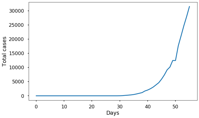
Since this data starts back in January, before the virus reached Italy, the number of cases at the beginning is zero. We can use the interval from day 30 to day 43 (inclusive) to try to fit \(\beta\), since this seems to be when the outbreak began to take off. Here it must be emphasized that the choice of this particular interval is somewhat arbitrary; different choices will give somewhat different values for \(\beta\).
def exponential_fit(cases,start,length):

    def resid(beta):
        prediction = cases[start]*np.exp(beta*(dd-start))
        return prediction[start:start+length]-cases[start:start+length]

    soln = optimize.least_squares(resid,0.2)
    beta = soln.x[0]
    print('Estimated value of beta: {:.3f}'.format(beta))
    return beta
Let’s see how well this value predicts the data:
def plot_fit(cases,start,end=56):
    length=end-start
    plt.plot(cases)
    beta = exponential_fit(cases,start,length)
    prediction = cases[start]*np.exp(beta*(dd-start))
    plt.plot(dd[start:start+length],prediction[start:start+length],'--k');
    plt.legend(['Data','fit']);
    plt.xlabel('Days'); plt.ylabel('Total cases');
    return beta

beta = plot_fit(total_cases,start=35,end=49)
plt.title('Italy');
Estimated value of beta: 0.247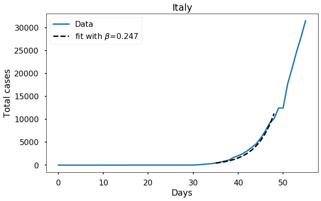
The fit seems reasonably good, over the interval we used. How well does it match if we plot the fit over the whole time interval?
start=35
plt.plot(total_cases)
dd = np.arange(len(days))
prediction = total_cases[start]*np.exp(beta*(dd-start))
plt.plot(dd[start:],prediction[start:],'--k');
plt.legend(['Data','fit']);
plt.xlabel('Days'); plt.ylabel('Total cases');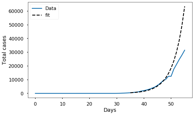
Clearly, the prediction is not accurate at later times. There are two main reasons for this:
We can resolve the first issue by using the full SIR model (instead of just exponential growth) to make predictions. The second issue is more complicated; we will try to deal with it in a later blog post.
To have more confidence in our value of \(\beta\), we can perform a similar fit with data from other regions, and see if we get a similar value. Next, let’s try fitting the data from the USA. Here’s the data:
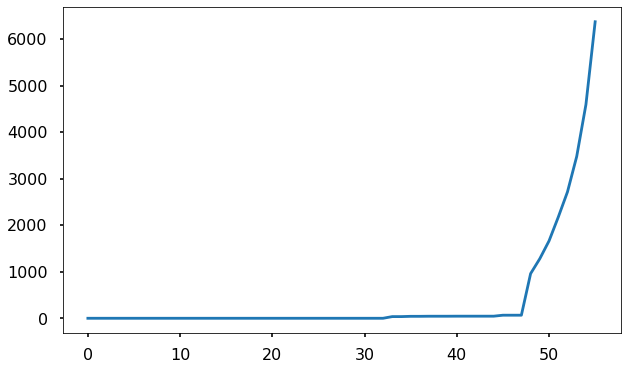
Notice that we only have about 1 week of meaningful data. Let’s try to fit an exponential to it:
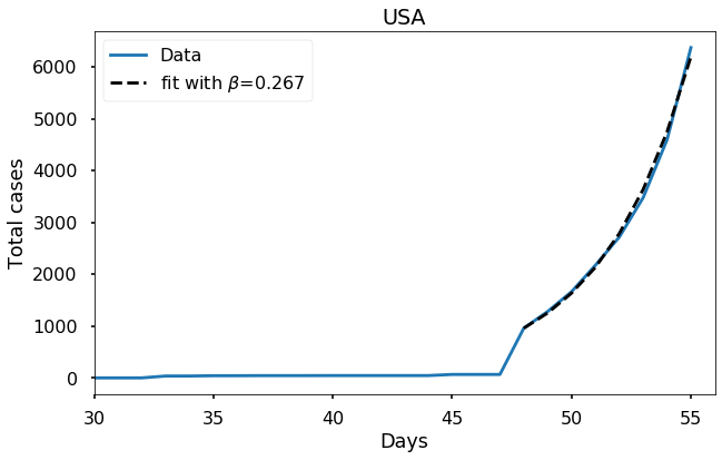
We get a fairly similar value for \(\beta\). Furthermore, the fit using this value seems to be pretty good.
Let’s look at the data from where it all started: Hubei province, China. Here it makes sense to start the fit from day zero of the JHU data set.
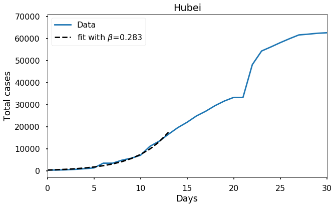
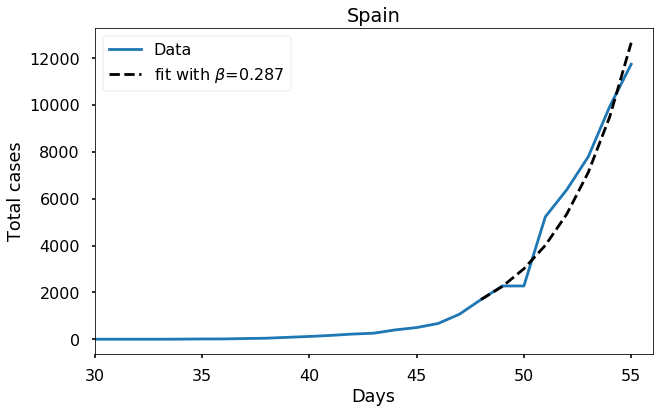
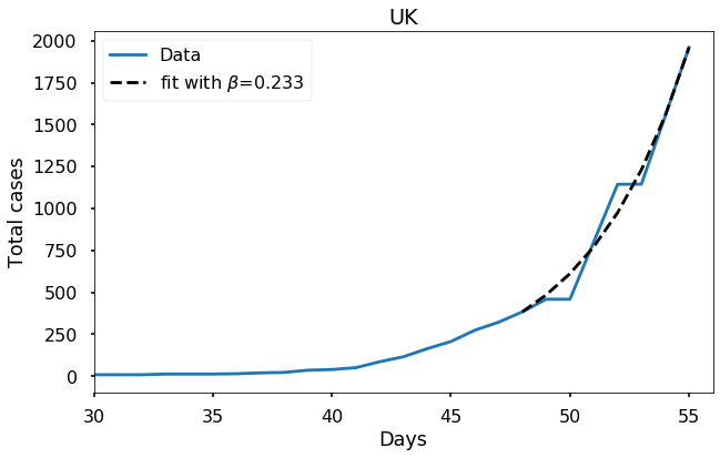
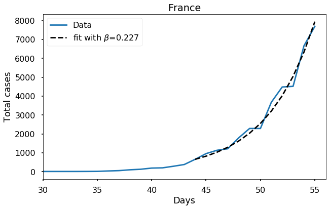
Each of these countries seems to fit the model reasonably well and to give a more or less similar value of \(\beta\), in the range \(0.22\) to \(0.29\). It would be wrong to feel completely confident about this value, or to try to extrapolate too much from such a short time interval of data, but the consistency of these results does seem to suggest that our estimate is meaningful.
Now let’s look at some countries that don’t fit this pattern.
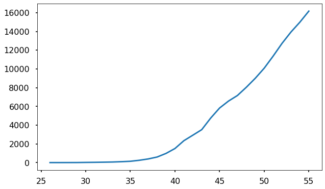
Here is the number of confirmed cases for Iran:
And here is Korea:
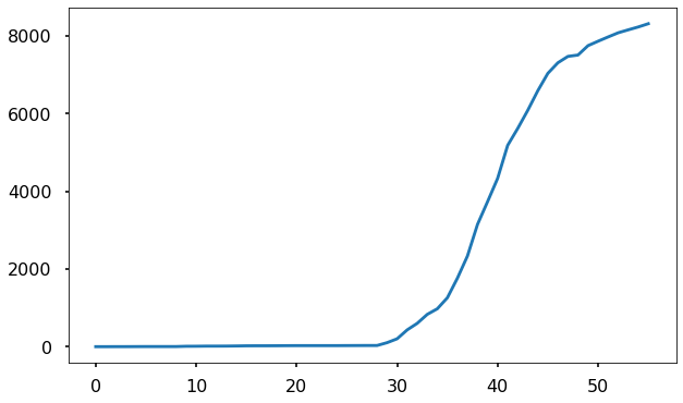
At a glance we can see that this data doesn’t follow the pattern of the previous countries. In Iran, after the first week, the growth seems to be linear. In Korea, the initial exponential growth eventually slows down drastically and is beginning to level off. This tells us that something we left out of our model must be at play.
In the case of Korea, it seems straightforward to understand what is going on. Korea has deployed the most extensive COVID-19 testing system in the world, with over 270,000 people tested to date. This is combined with an extensive effort to isolate infected people and those they have been in recent contact with. Essentially, South Korea has reduced the value of \(\beta\). Based on our earlier analysis, to prevent future exponential growth, they will need to keep \(\beta\) down to approximately the value of \(\gamma\) or less. If we believe that \(\gamma \approx 0.05\) and \(\beta \approx 0.25\), this means reducing the amount of human contact by infected people by five times.
Iran’s case is at first more puzzling, since the testing and quarantine measures there have not been exceptional compared to countries like Italy and Spain. Instead, there are strong suspicions that the official numbers from Iran are wildly inaccurate and the real number of cases (and deaths) is drastically higher than what is reported.
Before we go finish, it’s important to understand the limitations of the data we’re working with and the technique we have used. Most importantly, the numbers we have certainly do not represent the real number of infected individuals. That’s because many infected individuals are never tested for the virus. This is especially true for diseases like COVID-19 in which the majority of cases are mild and do not require professional medical care. Estimates I have seen claim that only about 10-20% of all cases are detected.
If we assume that the fraction of cases that are actually detected is constant over time, then this discrepancy does not hinder our ability to estimate \(\beta\), since dividing the initial and final number of infected by the same constant will lead to the same estimate of \(\beta\) that would be obtained if we counted all the cases. However, it’s clear that in many places this factor changes over time as a country starts doing more and more testing. This would cause the number of reported cases to grow even faster than the real number. This is most likely occurring, for instance, in the US where previously many individuals with symptoms were not tested due to a lack of test availability.
Another issue is that in some cases governments may be intentionally hiding the true number of infections. As we have seen, this is likely the case in Iran.
Finally, mitigation strategies may already be in place and influencing the rate of spread in some countries, even in the early days of outbreak. This would lead to us underestimating the natural value of \(\beta\).
What we can take away from this analysis are the rough estimates for the SIR parameters:
\[\gamma \approx 0.05\] \[\beta \approx 0.25.\]
Notice that the behavior in this initial phase of the epidemic that we have focused on is very similar to the simple behavior we considered at the start of the first post. There, the number of infected individuals doubled each day, but we knew that was unrealistic. Here, the number of infected individuals doubles every few days. How many days does it take for the number to double? If it takes \(m\) days for the number of cases to double, then we have
\[ e^{\beta m} = 2 \]
so \(m = \log(2)/\beta\) where \(\log\) means the natural logarithm. For \(\beta=0.25\), this gives a doubling time of about 2.8 days. This growth will slow down somewhat after the first couple of weeks for reasons we have already discussed.
It should be emphasized that the value of \(\beta\) here is what we expect in the absence of mitigation strategies. In later posts, we’ll look at what these values mean for the future spread of the epidemic, and what the potential effect of mitigation may be.
In the Jupyter notebook for this post there is an interactive setup where you can make your own fits to the data from a variety of regions.
Click here to go to the next post, in which we use what we’ve found to predict the future.