This post is the first in a series in which we’ll use a simple but effective mathematical model to predict the ongoing Coronavirus outbreak. As I write, the number of officially confirmed global cases is just under 200,000 and many schools and workplaces all over the world have closed in order to slow its spread. If you’re like me, you’re wondering:
My claim is that we can reach some reasonable approximate answers using straightforward mathematics. Math is quite effective at predicting the average behavior of large groups, and a little math can go a long way in telling us what will happen next with COVID-19. My goal here is to help you make and understand those predictions with little more than high school mathematics.
Disclaimer: I am not an epidemiologist and I make no guarantees about the predictions we’ll arrive at here. By reading this you agree not to sue me. What I write here does not reflect the opinion of my employer or anyone else.
Each post in this series is written in a Jupyter notebook, which you can download and experiment with yourself if you are so inclined. The notebook for this first post is here
An infectious disease spreads from one individual to another. Consider the following simple model:
How quickly does the number of infected individuals grow?
1, 2, 4, 8, 16, …
On each day, the number of infected doubles! How many days would it take for everyone on earth to be infected?
This is not a reasonable model for any of the diseases we know of. Of course, the rate of new infections per infected person (1 per day) was an arbitrary choice and real values are likely to be smaller. What other effects are missing from this model?
Those two factors are vital to understanding the true dynamics of epidemics. Of course, there are many other important details we have left out; for instance:
All of these effects (and many others) will influence the spread of the disease. A model that tries to incorporate them all would be very complex.
One of the simplest but most relevant models is based on the idea that the population consists of three groups:
When we write \(S(t)\), we mean that the number of susceptible individuals (\(S\)) is given as a function of time (\(t\)). We can’t write down this function exactly; instead it will be described by a differential equation. Now, differential equations are a bit like whale sharks: they sound scary at first, but in reality they are simple and friendly creatures.
A differential equation is just a description of how some quantity changes. In this case, we will have three differential equations, describing the rate of change of \(S\), \(I\), and \(R\). The idea is that susceptible people can become infected and infected people can become recovered:
\[ S \to I \to R\]
To define differential equations for the three groups, we only need to determine the rate at which each of these transitions occurs.
In our first simple model, we assumed the rate of infection was proportional to the number of infected. This is very reasonable, but for someone new to become infected we need both an infected individual and a susceptible one. If we imagine that people encounter each other randomly at some rate \(\beta\), then the rate of new infections is just the number of infected multiplied by the probability of encountering a susceptible individual:
\[ \frac{dI}{dt} = \beta I \frac{S}{N}. \]
Here \(N=S+I+R\) is the total population, so \(S/N\) is the probability that a randomly chosen individual is susceptible. This is probably the most complicated point of our discussion, so take some time to think about it until it makes sense to you.
Of course, since new infected people were previously susceptible, the number of susceptible individuals must decrease at the same rate:
\[ \frac{dS}{dt} = -\beta I \frac{S}{N}. \]
The other transition is from infected to recovered. A proper model for this should involve a time delay, since (for many diseases) new infected individuals typically become recovered after a certain interval of time. For instance, with the flu or the new Coronavirus, the number of new recovered individuals might depend on how many became infected about one or two weeks ago. Incorporating such an effect would lead to a more complicated model known as a delay differential equation.
Instead, we will simply assume that over any time interval, a certain fraction of the infected become recovered. Denoting the recovery rate by \(\gamma\), we have
\[ \frac{dR}{dt} = \gamma I. \]
The number of infected must decrease at the same rate, so we must modify our differential equation for \(I(t)\) to read
\[ \frac{dI}{dt} = \beta I \frac{S}{N}-\gamma I. \]
Taking these three equations together, we have
\[\begin{align} \frac{dS}{dt} & = -\beta I \frac{S}{N} \\ \frac{dI}{dt} & = \beta I \frac{S}{N}-\gamma I \\ \frac{dR}{dt} & = \gamma I \end{align}\]
Notice that if we add the 3 equations together, we get
\[ \frac{dN}{dt} = 0. \]
What do \(\beta\) and \(\gamma\) really mean? We can think of \(\beta\) as the number of others that one infected person encounters per unit time, and \(\gamma^{-1}\) as the typical time from infection to recovery. So the number of new infections generated by one infected individual is, on average, \[\beta/\gamma = R_0,\] the basic reproduction number.
Notice that \(S(t)\) can only decrease and \(R(t)\) can only increase, but \(I(t)\) may increase or decrease. A key question is, under what conditions will \(I(t)\) increase? This will tell us whether a small number of cases could become an epidemic.
We can write
\[ \frac{dI}{dt} = \left(\beta \frac{S}{N}-\gamma \right) I \]
from which we see that \(I(t)\) grows if \[\beta S/N > \gamma.\]
\[ \frac{dI}{dt} = \left(\beta \frac{S}{N}-\gamma \right) I \]
Initially in a population we have \[S/N \approx 1,\]
so an epidemic of some size can occur if \(\beta > \gamma\). As the epidemic grows, the ratio \(S/N\) becomes smaller, so eventually the spread slows down.
What fraction of the population must been infected before \(I(t)\) will start to decrease?
The epidemic will begin to subside when \[S/N = (\beta/\gamma)^{-1} = R_0^{-1}.\]
This determines the infection peak. After this point, there will still be new infections but the overall number of infected will decrease.
So what does an epidemic look like, using the SIR model? We can easily compute the solution using standard numerical methods; I’ve omitted the code here since I want to focus on the model, but feel free to look at the original Jupyter notebook with code and modify the parameters yourself.
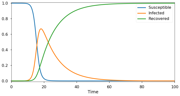
Here I’ve set \(N=1\) so the numbers on the vertical axis represent a fraction of the current population. Initially, only a tiny fraction is infected while the remainder is susceptible. The plot above shows the typical behavior of an epidemic: an initial rapid exponential spread, until much of the population is infected or recovered, at which point the number of infections begins to decline.
According to our analysis above, the number of infections should begin to decrease when the susceptible fraction \(S/N\) is equal to \(\gamma/\beta\). Here I’ve taken \(\beta=1\) and \(\gamma=1/10\), so the infection peak should occur when the susceptible population has dropped to 1/10. Let’s check:
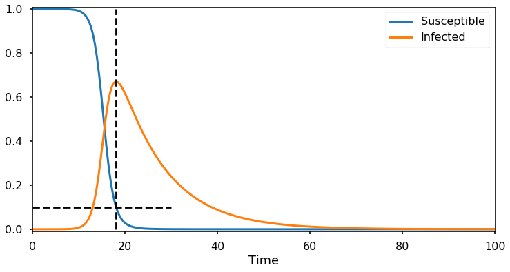
The results are in perfect agreement with what we predicted. In the original notebook there is an interactive model where you can adjust the parameters and see the results.
![]()
Click here to go to the next post, in which we look at real-world data to estimate the values of \(\beta\) and \(\gamma\).