A multiscale model for weakly nonlinear shallow water waves over periodic bathymetry
Abstract
We study the behavior of shallow water waves over periodically-varying bathymetry, based on the first-order hyperbolic Saint-Venant equations. Although solutions of this system are known to generally exhibit wave breaking, numerical experiments suggest a different behavior in the presence of periodic bathymetry. Starting from the first-order variable-coefficient hyperbolic system, we apply a multiple-scale perturbation approach in order to derive a system of constant-coefficient high-order partial differential equations whose solution approximates that of the original system. The high-order system turns out to be dispersive and exhibits solitary-wave formation, in close agreement with direct numerical simulations of the original system. We show that the constant-coefficient homogenized system can be used to study the properties of solitary waves and to conduct efficient numerical simulations.
Abstract of the arXiv version, arXiv:2311.02603.
Code and data
Reproducibility repository: https://github.com/ketch/shallow_water_bathymetry_effective_medium_RR
Animations
The question
Waves in shallow water are usually modeled by the shallow water (Saint-Venant) equations, which track the water depth and the depth-averaged velocity. Over a flat bottom, these equations predict that any hump of water eventually steepens until its front becomes vertical, like a breaking wave. After that, the hump spreads into a triangular shape (an “N-wave”) and slowly decays.
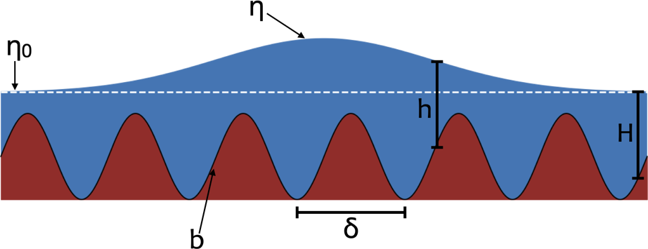
What happens if the bottom is not flat but has a repeating pattern of ridges and troughs? In these animations the bottom alternates between depths of 1 m and 0.3 m every half meter, and the water starts at rest with a smooth hump a few centimeters high. The hump splits into a left-going and a right-going wave; the animations follow the right-going one.
Flat versus periodic bottom
The dashed line shows the wave over a flat bottom: its front steepens into a vertical jump and the wave takes on the triangular N-wave shape. The solid line shows the same initial hump over the periodic bottom. Instead of breaking, it separates into a series of smooth, separate peaks.
Solitary waves
Running the periodic-bottom case longer shows that the peaks keep their shape and travel at different speeds, with the tallest in front. Waves like this, which hold their shape as they travel, are called solitary waves. They are typical of dispersive wave equations, in which waves of different lengths travel at different speeds, but the shallow water equations over a flat bottom are not dispersive. The periodic bottom supplies the dispersion.
A closer look
The same simulation near the end of the run, with frames much closer together in time. On this time scale you can see the wave shapes change rapidly as they pass over each step in the bottom, and a pattern of small ripples behind them.
An effective model
The main result of the paper is a set of homogenized equations: equations with constant coefficients, which no longer involve the detailed shape of the bottom, but whose solutions approximate the averaged behavior of the waves. The derivation produces a series of corrections in powers of \(\delta\), the period of the bottom relative to the length of the waves; keeping terms up to \(\delta^3\) or up to \(\delta^5\) gives two versions of the model. Both contain dispersive terms, which explains where the solitary waves come from.
This animation compares the shallow water solution with the two homogenized models. Both match well at first; over time the waves of the \(\delta^3\) model run ahead, while the \(\delta^5\) model stays close to the shallow water solution. The homogenized equations are also much cheaper to solve: for this problem the paper reports a speedup of about 200 times.